SatTech2.0
Product Objective
Generación de ficheros¿Cómo realizar un seguimiento eficiente de los cultivos?
The objective of SatTech2.0 is:
Monitor the entirety of an operation without cloud interference.
Detect problem plots weekly.
Analysis of the reasons for these problems.
Monitoring of crop water requirements.
Carrying out actions and recording them to analyze their impact.
File generation of reports and GIS application files for variable-rate application.
Display of biomass evolutions.
Application for information visualization and sample collection.
Information Sources
The SatTech 2.0 product obtains information from Sentinel-2 satellite for multispectral information, Sentinel-1 for radar information, and from a global network of weather stations for meteorological information.
Frequency
The Sentinel-2 satellite has a revisit period of five days. The Sentinel-1 satellite has an approximate period between six and twelve days depending on the world region. The Landsat-9 satellite has an approximate period between ten and fifteen days depending on the world region. The Planet satellite has an approximate period between one and two days depending on the world region. The meteorological information collects hourly data.
Layers
Below are the main layers and their derived information.
RGB
The RGB layer is generated with the combination of Red, Green, and Blue bands and allows viewing the field in visible light. This layer is interesting for having an aerial view of the crop state. No statistics are calculated based on this layer.
Vegetative Vigor (NDVI, LUVI)
Vegetative Vigor (NDVI)
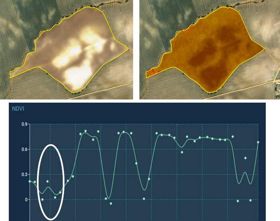
The NDVI (Normalized Difference Vegetation Index) provides information about the amount of photosynthesis that plants are producing. It is calculated using multispectral images that capture how plants reflect and absorb light waves of different wavelengths. This index provides information about the radiometric behavior of vegetation, related to photosynthetic activity and plant leaf structure, allowing determination of plant vigor.
An NDVI value above 0.65 in mid-season is good for most crops, but values in that range at the beginning may indicate areas with weeds (or digitization problems); similarly, this value at the end of the cycle may indicate that the plant is not yet ready for harvest. On the contrary, an NDVI value of 0.3 or lower is positive both at the beginning and end of the season. By clicking on the ‘i’ you will see the NDVI range legend.
This layer is complemented by two more, Vegetative Vigor (NDVI) - High Vigor and Vegetative Vigor (NDVI) - Early Phases, which show the previous index but with ranges limited to different moments of crop development.
This layer is available for LANDSAT and PLANET

You will see that for values below 0.25, Layers identifies as ‘Soil’ and colors in brown. There is also a cloud filter that colors in white those areas of the plot that may be affected by clouds. This filter is not infallible, so we recommend reviewing the RGB layer.

Maximum NDVI Vigor
The Maximum NDVI layers give us an idea of how NDVI has evolved throughout the cycle and allow us to study when a problematic area is structural or when there may be a specific problem in this campaign and where we can focus (diseases, pests, irrigation problems, etc.).

We will find them in two formats: Maximum vigor in 1 year and Maximum vigor in two months.

NDVI Variability
In the Dashboard, you will find NDVI Variability statistics. This parameter, which mathematically is the standard deviation of the plot’s NDVI, is a value of intra-plot heterogeneity. A low variability value indicates a homogeneous plot, while a high variability value may indicate problems with weeds, diseases, irrigation issues, etc.
Our recommendation is that you review weekly the analytical evolution of the mean NDVI and mean Variability at an analytical level in all your plots in the Dashboard, and then use the map to determine which areas need your attention the most that week.
You can see this evolution at a spatial level by dragging one of the satellite ‘dots’ with the date you want to compare over the date you want to compare it with.
Once in the field, we encourage you to use the Layers Application on your mobile to take a georeferenced photograph.
You have a new satellite image available approximately every 5 days.
Vegetative Vigor (LUVI)
The LUVI (Layers Unified Vegetation Index) is a layer where we unify the NDVI and Variability from different sensors to simplify the results into a single one.
LUVI is created by unifying Sentinel 2, Landsat 9, and Planet sensors (the latter for users who have it active), achieving a single data flow.
The LUVI variability is shown as the initial layer when opening Layers, assigning a color to each plot based on the variability presented by the crop. Therefore, this layer helps us identify plots where some problem may be occurring (lack of plants, development problems, pests, diseases, etc.)

To identify these plots more easily, a legend is attached with 4 variability ranges and an extra one to indicate lack of data (indicating that in the last 30 days there has been no cloud-free scene from any satellite).

Vegetative Moisture (NDMI)
The NDMI is a multispectral index similar to NDVI but includes SWIR (short-wave infrared) information, a band that allows capturing leaf moisture information.

The NDMI is sensitive to leaf moisture values and is commonly used to find irrigation problems.
This layer is available for LANDSAT and PLANET
Nitrogen-Chlorophyll (NDRE)
The NDRE is a multispectral index similar to NDVI but more sensitive to crops with higher vigor and chlorophylls. Often, the amount of chlorophylls is related to leaf nitrogen, hence the name of the layer.

It is sometimes used as a plant ‘health index’ to find problems in the crop. Low values may reflect long periods of water stress due to excess or deficiency.
Soil Texture
The Soil Texture layer indicates, under bare soil conditions, the distribution of different soil types that appear in our plot, classified generically (very sandy, sandy, loamy, and clayey), defining the soil’s capacity to retain water and nutrients, as well as their availability for plants, their temperature (cold or warm soils), the biological activity of microorganisms present in the soil, and its possible susceptibility to cryptogamic diseases (alternaria, anthracnose, botrytis, nematodes…). This layer is based on information from the Sentinel-2 satellite and its relationship with our own database, which has proven to be widely valid for high-level analysis as documented in available literature and improvements applied by the HEMAV team. To know the exact distribution of soil textures, sampling is necessary; we recommend interested parties to consult the SoilTech section.
How does the texture layer work?
The texture layer analyzes soil moisture variability through satellite imagery on vegetation-free soil, and applies a conversion process to transform these values into clay percentage contents, which are then classified into low, medium, or high levels. To provide a numerical value of actual clay percentage present in the soil, the image should be taken under ideal conditions (aerated soil after rain or irrigation). Since it is not always possible to obtain an image under ideal conditions, and to avoid confusion, a qualitative classification is used, which still adequately defines and classifies soil diversity. The following example shows this circumstance, viewing the layer evolution at an ideal moment (left), where the clay percentage values used by the statistical model would be very similar to those we could achieve with laboratory analysis, and on the right the same plot days later, when the layer still defines the different soil types, but with numerical values further from those that would result from laboratory analysis:

When can I use this layer?:
On bare soil (without vegetation), under tempering conditions (with soil aerated after rain or irrigation) would be ideal, but also with dry soils. To locate the appropriate image, I can use one of the initial phases of a crop, just after applying pre-sowing/planting work, using the Layers dashboard to locate the best date, as shown in the following image. It is also advisable to apply the Layers NDVI layer over the plot, as it colors in brown the surface lacking vegetation, allowing us to verify that the image is suitable:
Avoid using an image with very wet or waterlogged soil. If there is a part of the plot that has been plowed and another that has not, this circumstance will be reflected, as the soil moisture content affects the layer, and when plowing, that moisture rises to the surface and is perceived by the satellite. This same case would occur if the image is taken when a pivot is irrigating, as the recently irrigated area is more humid, it would affect the efficiency of the layer, showing heterogeneity that does not really exist:

What can I use this layer for?:
• To perform directed soil nutrient sampling in a much more representative way.

• To locate suitable test areas where soil variability does not influence the conclusions.

• To locate varieties. In the case of crops like tomato or corn, long-cycle varieties are usually avoided in clay soils, and it is usually indicated to establish them in sandy areas. There are even crops like asparagus or strawberry that require very sandy soils to develop.
• To vary the seeding density based on the productive potential of my plot (supported by technician/farmer knowledge, yield maps, laboratory data…)
• To create irrigation designs appropriate to soil characteristics and improve its efficiency, saving water and energy while improving crop development and health.

Digital Elevation Model 2010-2015
A Digital Elevation Model is a three-dimensional representation of the earth’s surface. The DEM 2010-2015 layer is a static compilation that does not vary with date. It corresponds to the GLO-30 DEM dataset generated by different satellites of the COPERNICUS constellation in the period 2010-2015. This information can be very interesting for certain analyses; however, it is important to note that the data in this layer are fixed and do not allow, for example, evaluating surface leveling work.
Crop Growth
The Crop Growth layer, based on RADAR information, allows monitoring the crop regardless of cloud presence. To calculate it, we only use suitable orbits to ensure proper conditioning of radar information in its VH polarization.
The Vegetative Growth Variability shows crop homogeneity in a way similar to NDVI Variability but based this time on the Variability of radar information.
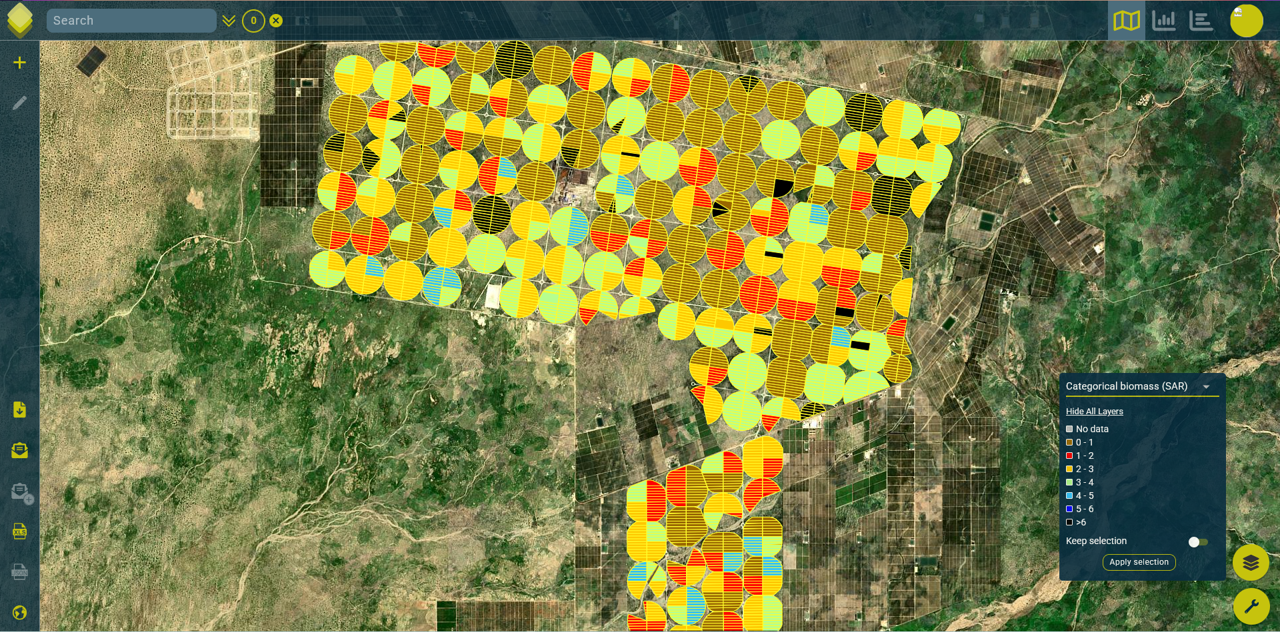
SAR BIOMASS
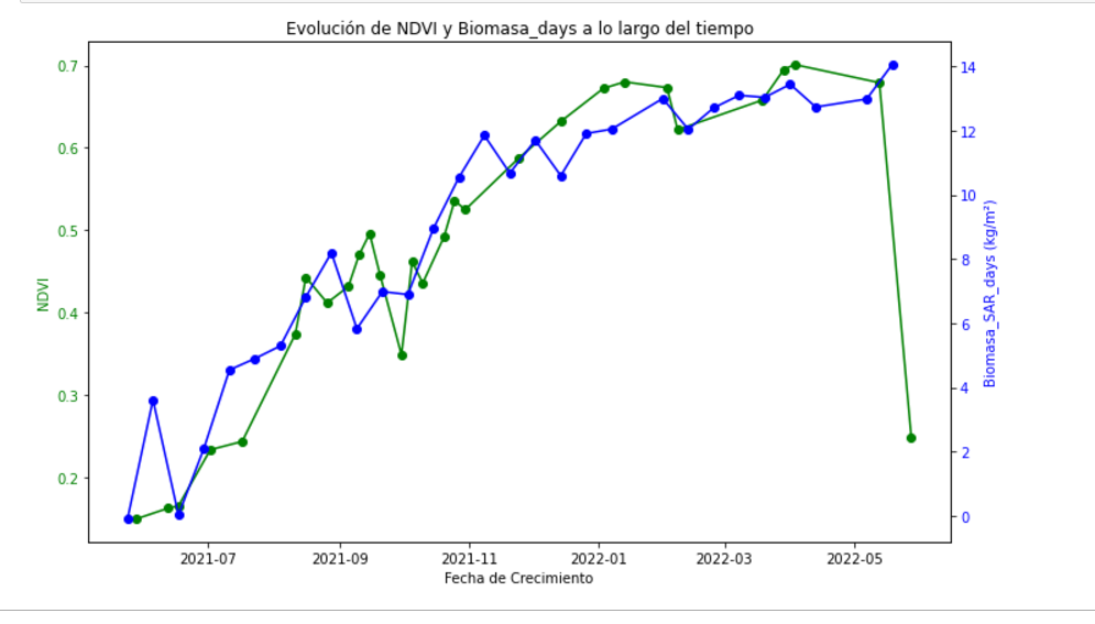
The SAR biomass layer is a global layer that estimates the amount of biomass in the field by relating crop days and radar value. In the case of sugarcane, the Biomass level theoretically approaches a value of Kg/m2. As can be seen in the following example image, the offered value has a good correlation with NDVI.
As this approximation is not precise in all situations, the layer is presented in categorical format (see table). It is important to note that the planting date or last cut is very relevant for this layer to provide the best information.
Legend:
CATEGORICAL SAR BIOMASS |
DESCRIPTION |
Color |
|---|---|---|
0 |
Soil - Very low |
Brown |
1 |
Low |
Red |
2 |
Low-medium |
Orange |
3 |
Medium |
Green |
4 |
Medium - high |
Light blue |
5 |
High |
Dark blue |
6 |
Cycle days out of range (+ 700 days) |
Black |
Historical productive potential (NDVI)
Historical productive potential (NDVI) is a layer developed by Hemav that allows analyzing the variability in the vegetative potential of each pixel that makes up the plot, by analyzing its behavior in previous years.

Based on the plot analysis after analyzing the NDVI behavior in the three years prior to the date when the layer is executed. The layer evaluates where NDVI has developed to a greater or lesser extent and assigns it a vegetative potential. This potential is based on the plot’s capacity pixel by pixel to generate biomass, given the strong relationship between biomass and the NDVI index.
VRA can be used to adapt seeding or fertilization levels to each differential zone using variable rate application machinery, improve irrigation system design by adapting it to detected variability, evaluate the best global agronomic management strategy based on greater representativeness, or adapt the most suitable varieties to each zone, among other examples. It is also useful for suppressing spatial variability when designing field trials or evaluating the overall quality of the plot.
This layer is especially indicated for plots that have homogeneous management, that is, that have traditionally been occupied by the same crop with very close sowing or planting dates. If the plot had very different sowing dates, was occupied by different crops, or had a part of the plot left uncultivated, these circumstances will be shown on the layer, usually appearing as well-defined geometric shapes that do not typically occur naturally, as shown in the following example, where a plot was occupied by two different crops and also maintained an uncultivated zone:

It is also important to keep in mind that the influence of a pest or disease on the crop in one of the years analyzed by the layer will have repercussions, potentially decreasing the productive potential in the affected area. If the plot currently does not have homogeneous management, but had it previously, we can activate the layer on that date to analyze the variability at that time.
Water stress (LWS)
Water stress (LWS) is an index developed by Hemav to analyze the crop’s water status, allowing the detection of deficit states at various levels.

It performs a comparison of the NDVI index to evaluate crop size and the NDMI index to analyze its moisture level. Traditionally, the NDMI index has been used to evaluate crop water status, but the values provided by this index are adequate or deficient depending on the crop’s development stage (A low NDMI index may be deficient if the crop has a large size, but adequate if it has a small size). By determining crop size through the NDVI value, we can easily determine whether the NDMI value is adequate or not.
It helps detect crop deficiencies caused by irrigation system failures or water supply calculations, but also allows us to evaluate water supply restrictions necessary in the final stages of the crop, aimed at drying the plant to prepare it for harvest. The use of intentional deficit irrigation in the final phases of sugarcane or beet to achieve an adequate sugar level, or to dry the grain in the case of irrigated cereals, can be adequately evaluated using this index.

In the previous image we can observe the effect of dirty or defective emitters on irrigation pivots.
Water deficit conditions produce physiological effects on the crop similar to pest or disease attacks when we perform analysis through satellite indices; therefore, situations detected by LWS may be due to a pathogen attack and not to a deficient irrigation level.
In the first weeks of cultivation, the influence of soil on the incipient crop could show deficit conditions without these being real, therefore it is advisable to evaluate the crop’s water status with LWS when it is large enough to be evaluated through satellite imagery.
Bare soil
This layer allows identifying bare soil on the surface of plots. It analyzes the plots in three categories:
Developed vegetation visible by satellite (Transparent): The layer classifies an area as vegetation and makes it transparent to remove it from the analysis.
Possible bare soil (Purple): The layer identifies areas with a medium probability of bare soil presence. These zones are colored in purple.
Bare soil (Red): The layer identifies areas with a high probability of Gaps presence and colors the surface in red.
Challenges in detecting Gaps with Sentinel-2:
• Pixel size (10x10 m): Makes it difficult to identify fine details within small plots or with underdeveloped crops. This size generates spectral mixing effects, where a pixel may contain both bare soil and vegetation, complicating precise separation.
• Shadows, soil colors, or moisture: Could alter spectral indices, reducing the reliability of classification.
• Plot boundaries and other elements: Plot boundaries, trees, paths, or buildings can blend within a pixel, making correct detection difficult and leading to erroneous classifications.
Possible weeds
This layer allows identifying areas potentially affected by weeds, as well as in some cases, other incidents. If the crop cycle is longer than 100 days and bare soil identification exceeds 35%, this calculation is applied only to the area identified as vegetation.
Analyzes the plots showing the category:
Possible weeds (Orange): The layer identifies areas with a high probability of weed presence, occasionally other incidents.
Challenges in detecting Weeds with Sentinel-2:
• Pixel size (10x10 m): Makes it difficult to distinguish scattered vegetation or vegetation mixed with the main crop.
• Spectral mixing: In areas where crops and weeds share a pixel, precise differentiation is complex.
• Similar spectral signatures: In certain growth stages, weeds and crops may have similar spectral characteristics, which affects accuracy.
• Plot boundaries and other elements: Plot boundaries, trees, paths, or buildings can blend within a pixel, making correct detection difficult and leading to erroneous classifications.
Combined use of Layers for sampling point selection
Below, we present an example of using Layers to carry out a plot analysis. Its utility lies in the ability to understand terrain variability, both from the soil perspective and the interaction between soil and crop. This type of analysis can be useful for locating samples (soil, production, etc.) and making them more representative, designing more effective irrigation plans (adapting irrigation sectors to soil type) or implementing variable applications, among other examples.

In the first image, we can observe different soil types (1), which seem to have an impact on productive potential (2). Soils with dark green tones, theoretically with lower clay content, seem to decrease potential production. When analyzing the complete development of the plot’s vegetative cover (3), a decrease in moisture is observed in these more sandy areas, probably due to less effective water retention. We have applied the Normalized Difference Vegetation Index (NDVI) to the early stages of crop development, and faster growth is evident in areas with theoretically higher clay content, probably due to the thermoregulatory effect of these soil types on seed germination, closely related to their water retention capacity.
Automatic Alert Report
Layers issues alerts to draw user attention to potential problems in their plots.
Automatic Alert Variability Report
These types of alerts arise from analyzing the existing variability in the crop present in the plot, with these alerts being of three types:
WARNING ACUM-LAS, or high crop variability alert
Layers analyzes the variability of an image to emit an alert if it is high enough to cause a low NDVI value (NDVI<0.4).
The alert arrives with this message and format:

This alert identifies highly heterogeneous plots for closer analysis, as pests, diseases, nutritional deficiencies, or other circumstances could be affecting the plant. The following images show some examples of the type of variability that Layers alerts about.

SUPER-LAS alerts, or crop evolution alerts in developed stages
Layers will analyze the variability of the latest available scene whenever the crop is developed (NDVI>0.4), and will compare it with the previous scene. If such variability increases, Layers will issue an alert.
The alert arrives with this message and format:

This alert allows us to identify possible:
• Fields that are being harvested.
• Sudden increases in crop variability due to pests, diseases, frost damage, etc.
In the examples shown below, we can observe some cases in this regard. On the left, an alert that would indicate that the plot varies because it begins to be harvested, while on the right it would show how a crop undergoes an alteration that decreases its NDVI. Although in this specific case it is due to the crop entering senescence, it could have also indicated a nutritional deficit, a pest or disease, etc.

INFER-LAS alerts, or crop evolution alerts in initial phases
Layers will analyze the variability of the latest available scene whenever the crop is in early growth stages (NDVI<0.4), and will compare it with the previous scene. If this variability increases, Layers will issue an alert.
The alert arrives with this message and format:

This alert allows us to identify possible:
• Presence of weeds or unwanted crops.
• Irregular start of crop growth and development.
The image shows an example of this type of alerts, where the current image (above) shows an increase in variability compared to the previous scene (below). This situation could reflect the incipient presence of weeds, or irregular crop development due to heterogeneous soil, sowing/planting failures, development of a residual crop, etc.
