PredTech
The Predictive product offers Crop Productivity and Quality Estimates.
This information is available in different formats depending on the needs of each entity.
Currently, HEMAV has an AI infrastructure that works for SUGAR CANE, CORN, SOYBEAN, COTTON, BEET, VINEYARD, and PALM crops.
The steps to access this service are as follows.
Input data to the model
The models must have as much input data as possible. These are divided into different blocks. With a total of 140 possible variables, associating the most important ones to each model according to the input data.
Customer data (real data)
This is the most important block. Models reflect the quality of the data. If there isn’t a sufficient amount of data, or if it lacks certain quality standards, when training the models they may not achieve the expected results.
In this section we refer to the data that we want the model to learn (production, quality…) and it is the starting point for data management (campaign start date, planting and harvest time).
This section has 40 possible data points to fill in, with the most important being:
external_reference_id: Unique identifier per installment.
season_label: Management grouping.
latitude: Georeferencing of the plot.
longitude: Georeferencing of the plot.
type_id: Crop
sub_type_id:
init_date: Campaign start date (start_date or plantation_date depending on the crop).
harvest_or_estimation_
cut_number: Cut number for crops such as sugarcane or palm.
production_per_hectare_real: Actual production obtained. Key variable for estimating the PRODUCTION model.
prodph_lastseason: Variable calculated by us, evaluating for that plot the production obtained in the previous season.
atr_real: Real ATR obtained. Key variable for ATR model estimation.
atr_lastseason: Variable calculated by us, always evaluating the production obtained in the previous season for that plot.
pol_real: Actual polarization obtained. Key variable for POL model estimation
sac_real: Real sucrose obtained. Key variable for SAC model estimation.
sac_lastseason: Variable calculated by us, always evaluating for that plot the production obtained in the previous season.
n_bunches_real: No. of bunches. Key variable for the N_BUNCHES model estimation.
plants_per_hectare: Number of plants per hectare. Important variable.
irrigation_type: Irrigation system used in the plot.
days: Growing days.
week: Growing week.
All these variables will define the quality of the requested model. This is why a series of reviews are carried out, which will be seen in the data review section.
Spectral data + radar
To the model’s dataset, the average value of the plot for the following spectral and radar values is incorporated for each date at a weekly level:
cloudcoverage: % of plot cloud cover on the day of visit. Only applicable for spectral parameters.
sigma0: Variable radar.
sigma0_std: Standard deviation of the radar variable. Shows the uniformity of the plot.
ndre: Nitrogen - chlorophyll index.
ndvi: Vegetation index.
ndvi_std: Standard deviation of the vegetation index.
b1: Sentinel 2 spectral bands.
b2: Sentinel 2 spectral bands.
b3: Sentinel 2 spectral bands.
b4: Sentinel 2 spectral bands.
b5: Sentinel 2 spectral bands.
b6: Sentinel 2 spectral bands.
b7: Sentinel 2 spectral bands.
b8: Sentinel 2 spectral bands.
b8a: Sentinel 2 spectral bands.
b9: Sentinel 2 spectral bands.
b11: Sentinel 2 spectral bands.
b12: Sentinel 2 spectral bands.
tcari_osavi: Soil-adjusted vegetation index that removes soil influence.
gndvi: Green-normalized difference vegetation index.
ccci: Chlorophyll index.
ndwi: Water status index (NDMI).
tcari: Index related to chlorophyll absorption.
OSAVI: The OSAVI vegetation index is a modified SAVI that also uses near-infrared and red spectral reflectance.
Spectral + radar data (temporal)
These are combinations of the previous variables processed to avoid cloud influence, indicating temporality or sudden data changes, since we work with accumulated data from the start of the campaign/planting, helping us to extract important indicators.
ndvi_smoothed: Ndvi working with a smoothing function removing the influence of cloud effects.
ndwi_smoothed: Ndwi (NDMI) working with a smoothing function removing the influence due to cloud effects.
ndvi_smoothed_temporal_max_diff: Maximum difference between weeks for the NDVI index.
ndwi_smoothed_temporal_max_diff: Maximum difference between weeks for the NDWI (NDMI) index.
ndvi_smoothed_max: Maximum NDVI value reached during the campaign.
ndwi_smoothed_max: Maximum NDWI value reached during the campaign.
ndvi_smoothed_temporal_mean_diff: Average difference between weeks for the NDVI index.
ndwi_smoothed_temporal_mean_diff: Mean difference between weeks for the NDWI (NDMI) index.
ndvi_std_temporal_max_diff: Maximum variability difference within the season.
sigma0_temporal_max_diff: Maximum difference of radar value within the campaign.
sigma0_max: Maximum radar value reached in the campaign.
sigma0_min: Minimum radar value reached in the campaign.
sigma0_temporal_mean_diff: Mean radar difference during the campaign.
sigma0_std_temporal_max_diff: Maximum radar difference during the campaign.
ndvi_growth_first_month: Maximum NDVI reached in the first month of the campaign.
ndwi_growth_first_month: Maximum NDWI (NDMI) reached in the first month of the campaign.
Climatological data
Climatological data is very important in the model as it indicates what the crop has been exposed to during the campaign. The variables we measure are the following:
pres: Mean pressure (mb).
slp: Mean sea level pressure (mb).
wind_spd: Average wind speed (Default m/s).
wind_gust_spd: Wind gust speed (m/s).
max_wind_spd: 2-minute maximum wind speed (m/s).
wind_dir: Average wind direction (degrees).
max_wind_dir: Direction of maximum 2-minute wind gust (degrees).
max_wind_ts: Time of maximum wind gust UTC (Unix Timestamp).
temp: Average temperature (Celsius by default).
max_temp: Maximum temperature (Celsius by default).
min_temp: Minimum temperature (Celsius by default).
max_temp_ts: Daily maximum temperature time UTC (Unix Timestamp).
min_temp_ts: Daily minimum temperature time UTC (Unix Timestamp).
rh: Mean relative humidity (%).
dewpt: Average dew point (Celsius by default).
clouds: Average cloud cover [satellite-based] (%).
precip: Accumulated precipitation (default mm).
precip_gpm: Accumulated precipitation [estimated by satellite/radar] (default in mm).
solar_rad: Average solar radiation (W/M^2)
t_solar_rad: Total solar radiation (W/M^2
ghi: Average global horizontal solar irradiance (W/m^2).
t_ghi: Total daily global horizontal solar irradiance (W/m^2) [Clear sky]
max_ghi: Maximum value of global horizontal solar irradiance during the day (W/m^2) [Clear sky]
dni: Average direct normal solar irradiance (W/m^2) [Clear sky]
t_dni: Total direct normal solar irradiance for the day (W/m^2) [Clear sky]
max_dni: Maximum direct normal solar radiation value for the day (W/m^2) [Clear sky]
dhi: Average diffuse horizontal solar irradiance (W/m^2) [Clear sky]
t_dhi: Total daily diffuse horizontal solar irradiance (W/m^2) [Clear sky]
max_dhi: Maximum diffuse horizontal solar irradiance value during the day (W/m^2) [Clear sky]
max_uv: Maximum UV index (0-11+)
Agro-climatic
We incorporate agro-climatic data due to their importance in the field of agriculture.
bulk_soil_density: Bulk soil density (kg/m^3).
skin_temp_max: Maximum skin temperature (C).
skin_temp_avg: Average skin temperature (C).
skin_temp_min: Minimum skin temperature (C).
temp_2m_avg: Average temperature at 2 meters (C).
precip: Accumulated precipitation (mm).
specific_humidity: Mean specific humidity (kg/kg).
evapotranspiration: Reference evapotranspiration - ET0 (mm).
pres_avg: Average surface pressure (mb).
wind_10m_spd_avg: Average wind speed at 10 meters (m/s).
dlwrf_avg: Average hourly downward longwave solar radiation (W/m^2 · H).
dlwrf_max: Maximum hourly downward long-wave solar radiation (W/m^2 · H).
dswrf_avg: Average hourly downward shortwave solar radiation (W/m^2 · H).
dswrf_max: Maximum hourly downward shortwave solar radiation (W/m^2 · H).
dlwrf_net: Net longwave solar radiation (W/m^2 · D)
dswrf_net: Net shortwave solar radiation (W/m^2 · D).
soilm_0_10cm: Average Soil moisture content 0 to 10 cm depth (mm).
soilm_10_40cm: Average Soil moisture content 10 to 40 cm depth (mm).
soilm_40_100cm: Average Soil moisture content 40 to 100 cm depth (mm).
soilm_100_200cm: Average Soil moisture content 100 to 200 cm depth (mm).
v_soilm_0_10cm: Average volumetric soil moisture content from 0 to 10 cm depth (fraction).
v_soilm_10_40cm: Average volumetric soil moisture content from 10 to 40 cm depth (fraction).
v_soilm_40_100cm: Average volumetric soil moisture content from 40 to 100 cm depth (fraction).
v_soilm_100_200cm: Average volumetric soil moisture content from 100 to 200 cm depth (fraction)
soilt_0_10cm: Average soil temperature at 0 to 10 cm depth (C).
soilt_10_40cm: Average soil temperature at 10 to 40 cm depth (C).
soilt_40_100cm: Average soil temperature at 40 to 100 cm depth (C).
soilt_100_200cm: Average soil temperature at 100 to 200 cm depth (C).
Processed climatological and agro-climatic data
gdd: Growing degree days accumulated with base temperature according to crop.
precip_temporal_max_diff: Maximum difference between weeks in precipitation during the campaign.
precip_max: Maximum precipitation value in a week.
evapotranspiration_max_diff: Maximum evapotranspiration difference between weeks during the campaign.
rh_max_diff: Maximum humidity difference between weeks during the campaign.
skin_temporal_max_min_diff: Maximum difference in maximum soil temperature between weeks during the campaign.
skin_temporal_min_min_diff: Maximum temperature difference in minimum soil temperature between weeks during the campaign.
gdd_min_diff: GDD difference between weeks during the campaign.
precip_first_month: Maximum precipitation reached during the first month of the campaign.
rh_first_month: Maximum humidity reached during the first month of the campaign.
skin_temp_max_first_month: Maximum soil temperature reached during the first month of the season.
solar_rad_first_month: Maximum solar radiation reached during the first month of campaign.
Data Review
The first step is calculating statistics for all the variables explained in the previous section. Once calculated, an automatic review of them is performed.
Currently, a summary report of this data review is generated, which can detect:
Temporal outliers: Such as problems with planting/harvest dates. Problems with predictor variables (anomalous estimations for a crop)
Global outliers: Detects any calculation issues across all explained variables.
All of this is represented in a summary report like the following:
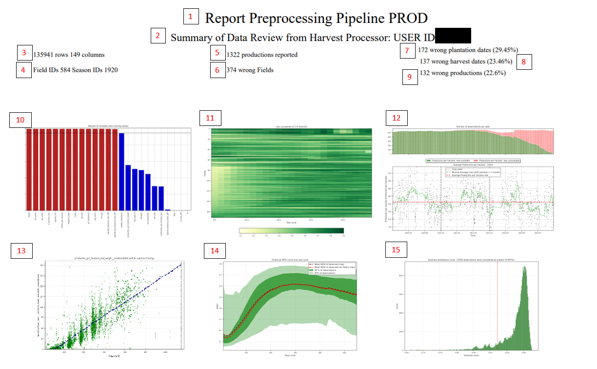
Enter the name of the report, it indicates that it is a preprocessing of the PROD variable.
Gives us information about the USER ID (be careful not to confuse user_id with customer_id or agrouser_id).
Shows the size of the dataframe.
Shows number of fields and seasons available for that client.
Number of actual data points for training (very important).
Number of data points that could be considered outliers.
Number of seasons with incorrect planting dates. Currently this is recorded if the NDVI in the first 30 days is greater than 0.4 (for “sugarcane”, “beetroot”, “soybean”, “corn”, “cotton”). (File attached in S3).
Number of records where the harvest date is considered incorrect (File attached in S3) taking into account the planting date (e.g., seasons that are too long or too short).
Number of real production data points that are considered outlier candidates, using two standard deviations above the moving average of the data on the days axis. (File attached in S3).
Graph showing the number of columns with missing data and % of missing data per variable.
NDVI evolution graph by cultivation days for season_ids with errors.
Evolution of production over time series. The upper graph shows the amount of data with actual production (green) compared to data without reported actual production (red). The lower graph shows the evolution of reported actual production.
Yield by cultivation days with limit axes to detect outliers based on time series data using population mean and two-thirds (2/3) of standard deviation over the moving average.
NDVI evolution by cultivation days smoothed by plant day-cycle.
Isolation forest: Shows us the distribution of scores in a histogram given by the algorithm, and the number of observations considered outliers. (https://scikit-learn.org/stable/modules/generated/sklearn.ensemble.IsolationForest.html)
All outlier candidates warn us about possible values that should not be introduced into the model, but this step is performed in the next section.
Model generation
Model generation is also performed automatically.
Currently, we have the automatic generation of 3 simultaneous models performing hyperparametrization techniques with the aim of obtaining the best model for the provided data.
After automatic training, a summary report of results evaluation is also generated:
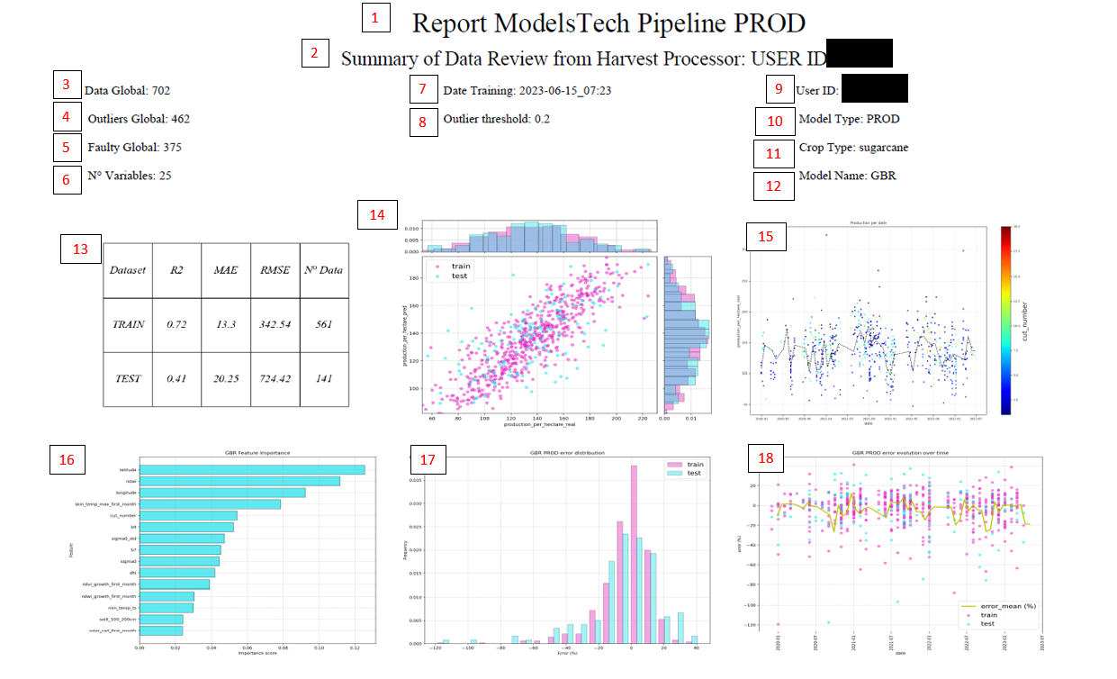
Report title.
Indicate the user of the model.
Data that finally enters the training.
Outliers detected with isolation forest
Number of outliers in preprocessing, as in “faulty_seasons_dict”
Number of variables that entered the model.
Training date.
The outlier_threshold that was set in the config.
Model user.
Model type.
Model training.
Model type with the best accuracy (RFR -> Random Forest Regressor (helps prevent overfitting); GBR -> Gradient Boosting Regressor (intermediate, but overfits more); XGBR -> eXtreme Gradient Boosting Regressor (overfits the most, but usually gives the best results)).
Summary table of accuracies.
Graph to check actual vs predicted data distinguishing between train and test.
Evolution of actual production over time.
Most important variables of the trained model.
Distribution of errors in train and test. If train and test are very different, then you should review what happened, and why the test data does not represent the training data.
Error distribution over time.
In addition to this summary report, you can also consult with your KAM/CPM interesting graphs for more in-depth data analysis within our production model manager (MLFLOW)
Generation of predictions
Once the data has been reviewed and trained, we use the generated model to make predictions in the campaign.
Predictions are updated on a weekly basis. To internally validate the results, we also generate reports to ensure everything is running correctly and we don’t detect strong anomalies.
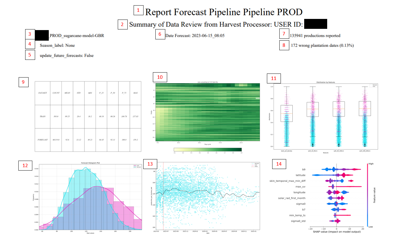
Report title.
Indicates the user that the prediction has been made.
Model type.
If any season_label filter has been used.
If it has been applied to update only future or all.
Prediction date.
Number of predictions generated (for each season_id there are multiple dates, hence the large number).
Plots that should have their planting date reviewed.
Summary table. Shows the distributions of the data used for training and the predicted data. It is normal that there will always be some deviation between the training mean and the forecast, since the training only takes the harvest date and the forecast takes everything.
Graph rescued from preprocessing to detect planting problems.
Distribution graph of the most important variables in the model, to observe the distribution of the model and the data to be predicted
Data frequency according to the value to predict, segmented by trained and predicted
Evolution of estimates over time, along with the data used to train the model (if there is data from the last year used to train it).
Variables con más importancia, como afectan sus valores para la predicción. La línea vertical indica el valor esperado (E(X)). Entonces, cada observación, tiene un valor para cada una de las variables. El gráfico de arriba indica cómo valores altos de esa variable (en color rojo), modifican la observación respecto al valor esperado. Por ejemplo, la variable más importante muestra que los valores rojos aumentan el valor de la predicción, respecto al valor esperado o lo que vendría a ser la media. En cambio, los colores azules, representan valores bajos de esa variable, y en la variable más importante se ve cómo valores bajos (color azul), hacen que la predicción sea más baja.